Evaluation of Sigma Labs’ in-situ process control system during Additive Manufacturing

Engineers at Sigma Labs Inc., Santa Fe, New Mexico, USA, recently performed an experiment to evaluate Quality Signatures™ using in-situ process control. This experiment was designed to establish a correlation between in-process dependent data mined from in-situ sensor raw trace signals, independent process input variables – for example laser power – and post-process dependent data measured during destructive metallographic testing for the porosity of as-built specimens.

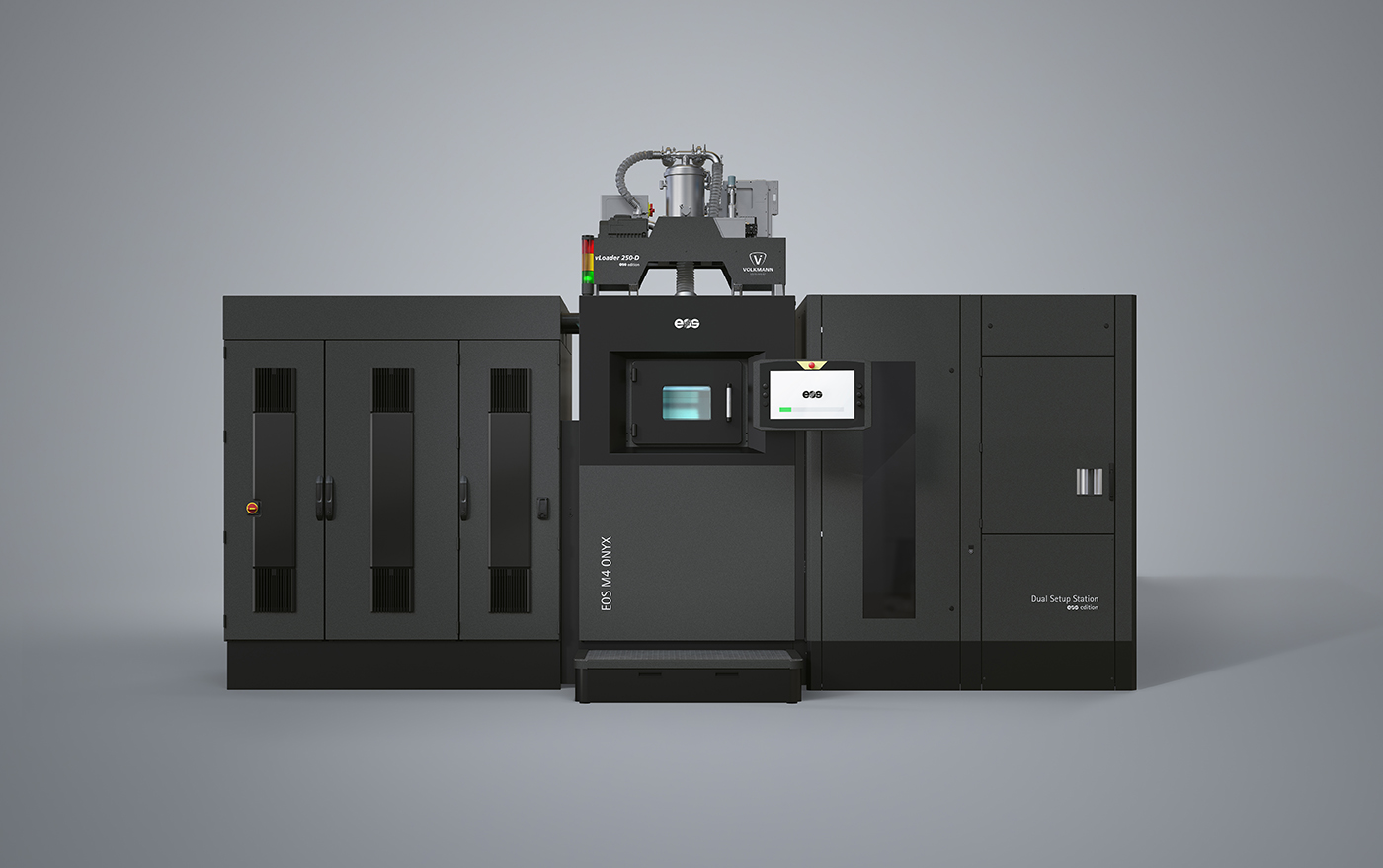
The metal powder used for these experiments was aluminium alloy AlSi10Mg. It had a particle size distribution (PSD) of 15-50 µm and was supplied by Valimet. All builds were performed using a standard EOS M290 Additive Manufacturing system integrated with Sigma’s PrintRite3D SENSORPAK^® system and PrintRite3D INSPECT^® software.

Four in-situ sensors were used during these experiments. The sensor types comprised non-contact, non-imaging optical sensors as well as non-contact thermal sensors. One sensor was a photodetector placed in a fixed, or Eulerian, frame of reference and positioned above the build plate. Its field of view (FOV) was of the entire build plate. A second photodetector was placed in a moving, or Lagrangian, frame of reference within the optics train. Its FOV was restricted to a narrow region immediately surrounding the melt pool. The third sensor was a high-speed, single wave length pyrometer, placed in a fixed frame of reference above the build plate and focused onto a 10 mm, right circular cylinder serving as a Process Control Specimen (PCS). Its FOV was 1 mm. The fourth sensor collects X and Y command signals from the scan head controller and is used to visualise in-process dependent data or In-Process Quality Metric™ (IPQM^®) data in a 3D point cloud. All sensor data was collected using PrintRite3D SENSORPAK’s high-speed data acquisition, running at 50kHz per channel, and subsequently analysed using the company’s PrintRite3D INSPECT.

Experimental approach

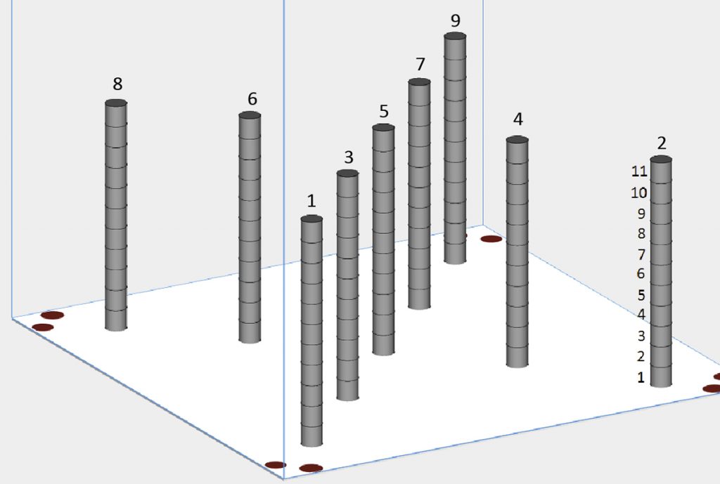
For this experiment, right circular cylinders 10 mm in diameter and 10 mm tall were built using the configuration shown in Fig. 1. A total of nine cylinders were built with one directly beneath the fixed pyrometer. The configuration was intentionally designed to space the specimens across the build plate and allow for the determination of spatial and temporal variation that may exist due to machine or sensor variability.

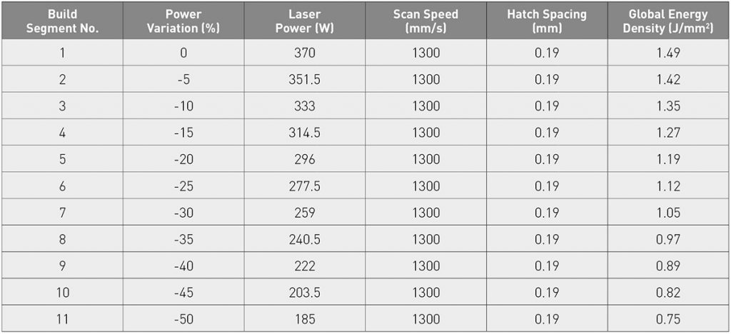
The starting or control parameters were suitable for lasing Al metal powder. Table 1 lists the control parameters and the ten different sets of processing parameters as well as the calculated Global Energy Density (GED) values. Layer thickness was held constant at 30 μm and each build segment contained 333 layers. The chamber atmosphere was argon and the build plate pre-heat temperature was 170°C.

Results

Data analysis: process control specimen

Univariate trend plots: melt pool level

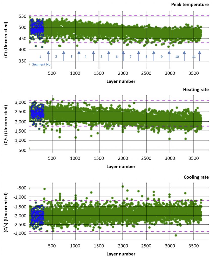
The trend plots in Figs. 2-3 were generated using Sigma’s standard PrintRite3D INSPECT software and algorithms using dependent in-process data mined from the high-speed pyrometer raw trace signal. The control data set (blue markers) used for this analysis was taken from build segment 1, layers 50 to 325. As stated, there were eleven vertical build segments, each containing 333 layers, and identified in Fig. 2 by blue arrows. Each trend plot was reported on a layer by layer basis and included a calculated +/- 3σ upper and lower control limit (UCL, LCL) represented as dashed lines.

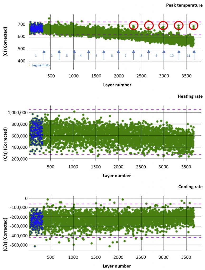
Fig. 2 comprises three trend plots of dependent in-process data that individually allowed the melt pool to be tracked according to its peak temperature, heating rate and cooling rate for a given layer. The melt pool dependent in-process data were mined at a fast time scale, e.g., microseconds (µs). By doing so, it was possible to infer changes in the melt pool geometry/volume associated with changes to independent process input variables, namely changes in laser power level. Each data point represents a single laser scan for a given layer. By doing so it is possible to track subtle changes to the melt pool which ultimately would be induced by other process disturbances such as presence of large powder particles or melt pool spatter, not necessarily changes to independent process input variables. Therefore, Sigma’s proprietary algorithms would allow for process disturbances to be distinguished from natural process variation.

In all three trend plots the dependent in-process data appeared to be normally distributed. Of interest is the drop in Peak Temperature as the build increased in the Z direction. This corresponded with a decrease in power levels as expected since the melt pool would be expected to reduce in size and maximum temperature with reductions in laser power. Of further note were the apparent natural data breaks (red circles) present because of standard upskin/downskin parametric changes visible around layers 3,300 and 3,700. These upskin/downskin parameter changes were pre-programmed into the EOS M290 and occurred between build segments since each segment was programmed as a separate part. Lastly, it is interesting to note that there was a shift in heating rate and cooling, which was also expected as power levels decreased.

A final comment should be made about the melt pool trend plots in Fig. 2. The Y-axes were labeled ‘corrected’ because the proprietary algorithms used by Sigma incorporated emissivity correction factors for the given material.

Univariate trend plots: layer level

It was also possible to mine the in-process pyrometer raw trace at a slower time scale for additional dependent in-process data and infer information about the bulk material’s response to the energy input such as defects associated with lack of fusion (LOF) or spherical porosity associated with keyholing.
In Fig. 3 similar trend plots were generated but this time displayed using thermal history information rolled up for the entire layer from melt pool level information. It is important to note that the layer level trend plots exhibit similar trends to those generated at a melt pool level. For example, there was a decrease in peak temperature, heating rate and cooling rate as the power levels were intentionally decreased.

Multivariate trend plot: melt pool level

It is convenient to represent multiple univariate trend plots in one trend plot while maintaining data continuity without the loss of process sensitivity or data integrity. Therefore, Sigma uses a proprietary multivariate analytics software engine to represent such trend plots. In Fig. 4, a Multi-Variate Statistical Process Control (MVSPC) trend plot combined the results for all univariate trend plots for melt pool information from Fig. 2, i.e., peak temperature, heating rate and cooling rate. This combined dependent in-process data was termed In-Process Quality Metric or IPQM. The Y-axis for the MVSPC trend plot in Fig. 4 is on a log scale because when a data point is flagged as an outlier it may in fact be a significant outlier and far from the normal distribution, hence it is convenient to display such data on a semi-log trend plot. For MVSPC trend plots there is only one control limit (blue dashed line) because the multivariate classifier control data set is defined by a single sided distribution, and it was established using a 95% confidence limit. This means that 95% of the data population lies within the boundary and 5% lies outside the boundary. The control limit is user definable and can be set between 90 and 99%.

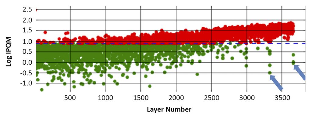
For the melt pool MVSPC trend plot in Fig. 4 there was an increasing trend in the IPQM values, which correlated with the parametric changes by segment observed in the univariate trend plots in Fig. 2. The MVSPC trend plot in Fig. 4 is a convenient way for a process engineer to quickly determine if the process is under control. If this were an actual build without intentional changes in laser power the operator would be alerted that the process had trended out of control. Lastly, as a confirmation of data continuity, Fig. 4 upskin/downskin parametric changes were still visible around layers 3,300 and 3,700 (blue arrows).

Multivariate trend plot: layer level

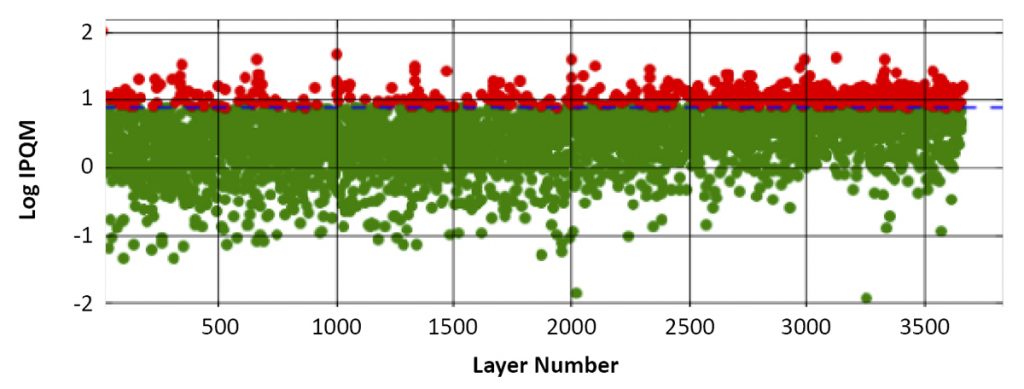
Fig. 5 is also a MVSPC trend plot which combined the results for all univariate trend plots for layer level information from Fig. 3, i.e., peak temperature, heating rate and cooling rate. For the layer level MVSPC trend plot in Fig. 5 it was observed that there was a slight increase in the IPQM values starting around layer 2,300 which correlated with the parametric changes by segment observed in the univariate trend plots in Fig. 3.

Data analysis: all specimens

Multivariate trend plots: part level

Fig. 6 contains a trend plot of in-process dependent data collected from both on-axis and off-axis photodetectors for an entire layer; it clearly captured the independent process input parameter changes by layer. All scans, for all parts for a layer are rolled up and plotted as a single data point for that layer. Then each test layer is compared to the control data set (displayed as the control limit/blue dashed line) and the resultant IPQM value is displayed on a log scale for ease of viewing. The results indicate that as the independent input variable (power level) was changed, there was a corresponding change in the in-process dependent variable (IPQM value).

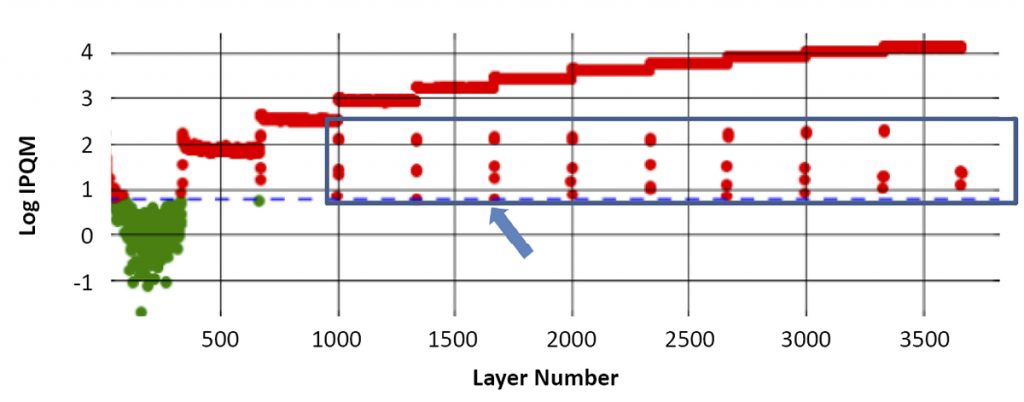
The intermittent points between each build section were the upskin and downskin scans (blue box) that were pre-programmed into the M290 between the completion of one build segment and the start of the next.

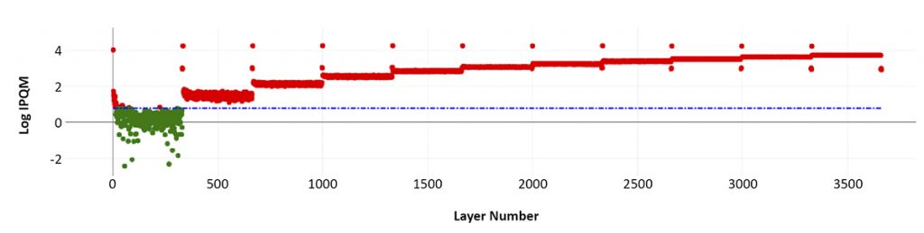
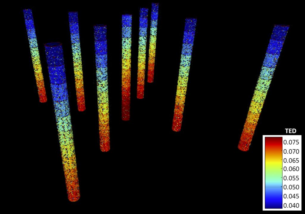
Fig. 7 contains a trend plot of the in-process data collected by the photodetectors for part 2, which is the process control specimen. Once again there were clear changes in the dependent in-process IPQM values in response to the intentional process parameter changes to laser power. Note the individual data points in between each build segment. These represent upskin and downskin parametric changes as compared to control parameter settings. Fig. 8 is a 3D point cloud visualisation of Sigma’s proprietary, quantitative In-Process Quality Metric known as Thermal Energy Density™ (TED™). TED comprises proprietary dependent in-process feature data mined from and calculated using photodetector raw trace signals from the melt pool. TED from the melt pool is summed over a single scan length, over the area of a layer or over the area of a part, resulting in an areal energy ‘density’. So, TED as it is calculated and displayed here corresponds to the part’s areal response to the input GED (laser power, travel speed, hatch spacing and overlap). Each vertical build segment has a different TED value assigned to it and correlates with intentional changes to independent process input variables for example changes in laser power level. TED can be expressed in units of power, time and distance.

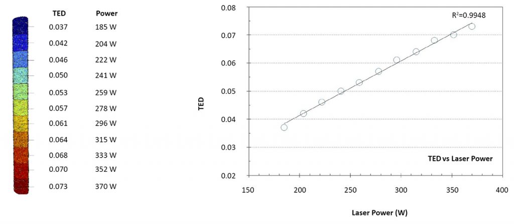
As a separate verification that Sigma’s TED metrics correlated with changes in laser power, Fig. 9 is a trend plot of TED as a function of laser power with visualisation of the process control specimen. It indicated that changes in Sigma’s TED metrics correlated with variations in laser power. An R² value of 0.9948 for the trendline indicated that the TED data is represented very well by a linear model.

Metallography and analysis

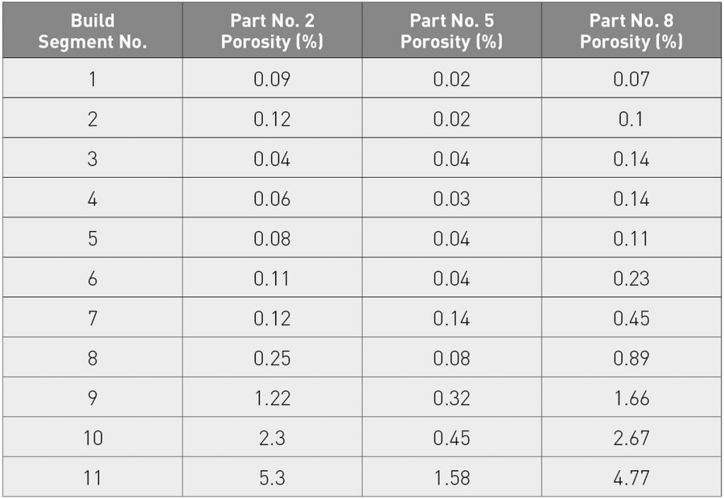
Metallographic services were provided by Metals Engineering and Testing Laboratories, Phoenix, Arizona, USA. Three specimens (parts 2, 5 and 8) were sectioned into two pieces, mounted and polished in accordance with ASTM E3. Once prepared, the specimens were examined in the as-polished condition from 20 to 500X magnification. Photomicrographs were taken at 50X magnification in the centre of each build segment for parts 2, 5 and 8. Image analysis was performed to quantify the (defect density) average areal percent porosity on a build segment basis. Table 2 contains metallographic results for porosity measurements.

Figs. 10, 11 and 12 are photomicrographs taken of cross sections made in the axial or Z direction of parts 2, 5 and 8, segments 1, 7 and 11, respectively. Each specimen was etched using Kellers Reagent to reveal individual melt (weld) pool beads.

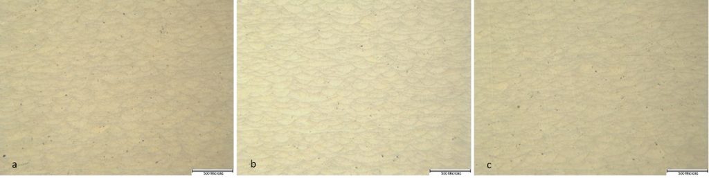
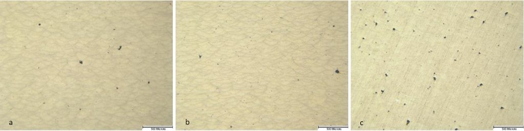
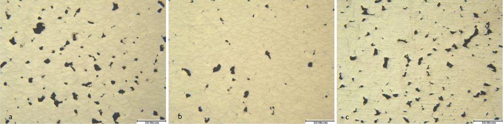
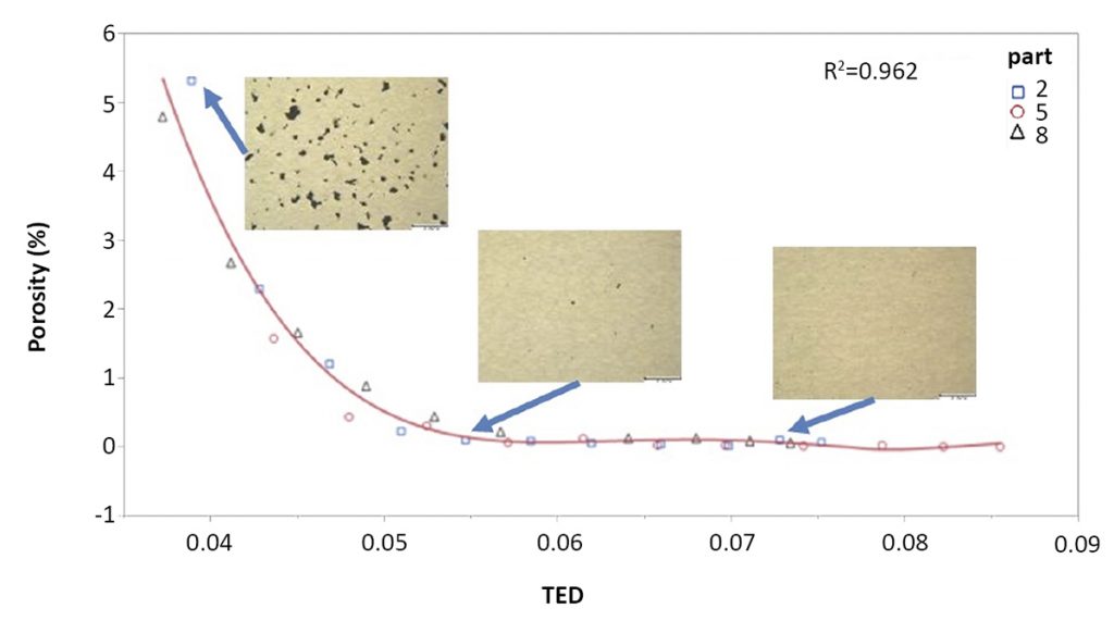
Fig. 13 is a plot of percent porosity measured versus TED for all 33 segments evaluated. An asymptotic relationship of percent porosity measured as a function of TED is present. Fig. 14 is a plot of laser power and TED as a function of percent porosity measured. An asymptotic relationship of percent porosity measured as a function of TED and power is present. Fig. 15 is a plot of TED and GED versus percent porosity. An asymptotic relationship is also present.

Summary

This experiment evaluated the sensitivity of the PrintRite3D INSPECT software and Sigma’s IPQM (TED) metric to changes in the independent process input parameter (laser power) on a layer by layer basis. Using this software and proprietary algorithms, that measure dependent in-process data captured from a pyrometer and photodetector raw trace signals, it is possible to infer effects of process disturbances on melt pool and bulk material thermal responses.

It was observed that thermal in-process dynamical trend data exhibited a Gaussian behaviour when analysed using the software’s IPQMs. Trend charts also contained a user defined upper control limit which enabled statistical process control capability on a layer basis. Using the TED IPQM and the on-axis photodetector in-process data for an entire layer, upskin and downskin scan locations were clearly visible. By analysing the TED metric, in relation to laser power and porosity, a strong correlation was observed.
In conclusion, Sigma’s IPQM TED metric represents a very good candidate for an In-Process Quality Metric of melt pool process disturbance for metal Additive Manufacturing.

Authors

Darren Beckett – Engineering Manager, Scott Betts – R&D Process Engineer, and Mark Cola – President & CTO
Sigma Labs, Inc.
3900 Paseo del Sol
Santa Fe, NM 87507
USA
Email: [email protected]

www.sigmalabsinc.com

Acknowledgements

The authors thank Dr R Bruce Madigan, Professor of Welding Engineering and Chair General Engineering Department Head, MontanaTech University, Butte, Montana, USA, for his valuable insight and technical review of this paper.

References

[1] 3D opportunity for quality assurance and parts qualification: Additive Manufacturing clears the bar, Deloitte University Press, 2015.

[2] Frazier, W.E, 2014, “Metal Additive Manufacturing: A Review”, Journal of Materials Engineering and Performance, 23:1917-1928.